Introduction
Accuracy and precision are fundamental characteristics of CUWB Systems. This application note provides empirical data to establish baseline performance expectations for CUWB deployments.
While the CUWB System is capable of highly precise positioning under ideal conditions, real-world environments and other constraints introduce variables that degrade this metric. However, the CUWB architecture allows users to balance accuracy and precision requirements with infrastructure cost and complexity.
To establish a shared terminology, it is critical to distinguish between two foundational concepts:
- Precision (Repeatability): The variation in the reported position of the Tag. High precision means low spatial noise.
- Accuracy (Truth): The deviation of the reported position from the actual physical location.
Accuracy is primarily a function of installation quality and environmental conditions rather than system tuning. Because the CUWB Engine relies on precise timing measurements, the following factors determine absolute accuracy:
- Anchor Density: The more Anchors in range of the Tag, the higher the accuracy that will be achieved. The CUWB system uses all Anchors in range of the Tag in the location solution.
- Anchor Survey: If the physical coordinates of an Anchor are measured incorrectly, every Tag location derived from that Anchor will contain a static bias.
- Line-of-Sight (LoS): Physical obstructions in Non-Line-of-Sight (NLoS) environments force signals to travel through or around barriers. This increase in path length or reduction in signal speed causes a Tag to appear more distant than its actual position. While the CUWB System includes advanced occlusion mitigation features to address these challenges, persistent NLoS conditions will degrade overall system performance.
- Device Placement: Inaccuracies can stem from site-specific variables, such as reflections and multipath interference caused by Anchors placed near RF-reflective materials or Tags tracked in close proximity to the ground.
While the CUWB Engine can mitigate some dynamic errors, static accuracy errors must be resolved through proper survey techniques, ensuring clear LoS where possible, or application-level adjustments of locations. See the Component Placement Guide for more information.
Precision is the primary performance characteristic that can be managed through system configuration. Poor precision manifests as ‘noise’ or ‘jitter’ in the position output. The goal of a high-performance deployment is to minimize the standard deviation of this noise to create a smooth, reliable position track. There are two primary techniques for improving precision through system design and CUWB features: mathematical smoothing and high Anchor density.
Smoothing
An effective and simple way to improve precision without adding infrastructure is oversampling, a technique where high-frequency location data is mathematically smoothed to reduce spatial noise.
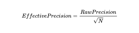
The Math of Averaging
In Line-of-Sight environments, UWB ranging error is widely accepted to follow a Gaussian (Normal) distribution. Gaussian noise is random, and as a consequence it tends to average out over time.
According to the Law of Large Numbers, the standard error of the mean decreases by the square root of the number of samples, N. For example, smoothing factors of 10 and 100 should theoretically result in a standard deviation improvement by a factor of roughly 3 and 10, respectively.
The CUWB System incorporates a simple average smoothing filter. A position is calculated at the nominal rate, but the output is smoothed over the last N samples.
Measured Performance - Smoothing
Test Environment: We conducted accuracy and precision testing in a medium-sized room of approximately 8 by 20 meters. The test deployment provided up to 24 ceiling-mounted Anchors and featured clear Line-of-Sight to Tags. Anchor placements in this setup were optimized for XY tracking; Z-axis data is not provided.
Ideally, real-world data would perfectly track the curve described in the previous section. However, physical environments introduce time-correlated noise such as multipath interference and reflections that can persist longer than a single sample duration, particularly when a Tag remains stationary. Because these consecutive samples are not purely independent random events, the error resists simple averaging, resulting in a measured standard deviation that improves significantly but remains higher than the theoretical mathematical ideal.
Despite these physical realities, the data shows that oversampling transforms the system’s precision performance.
 |
 |
 |
|---|---|---|
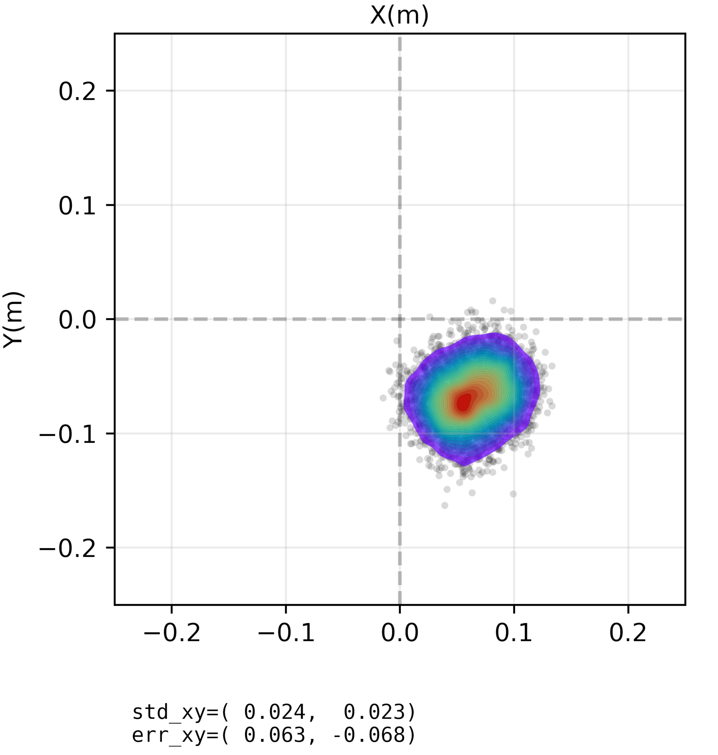
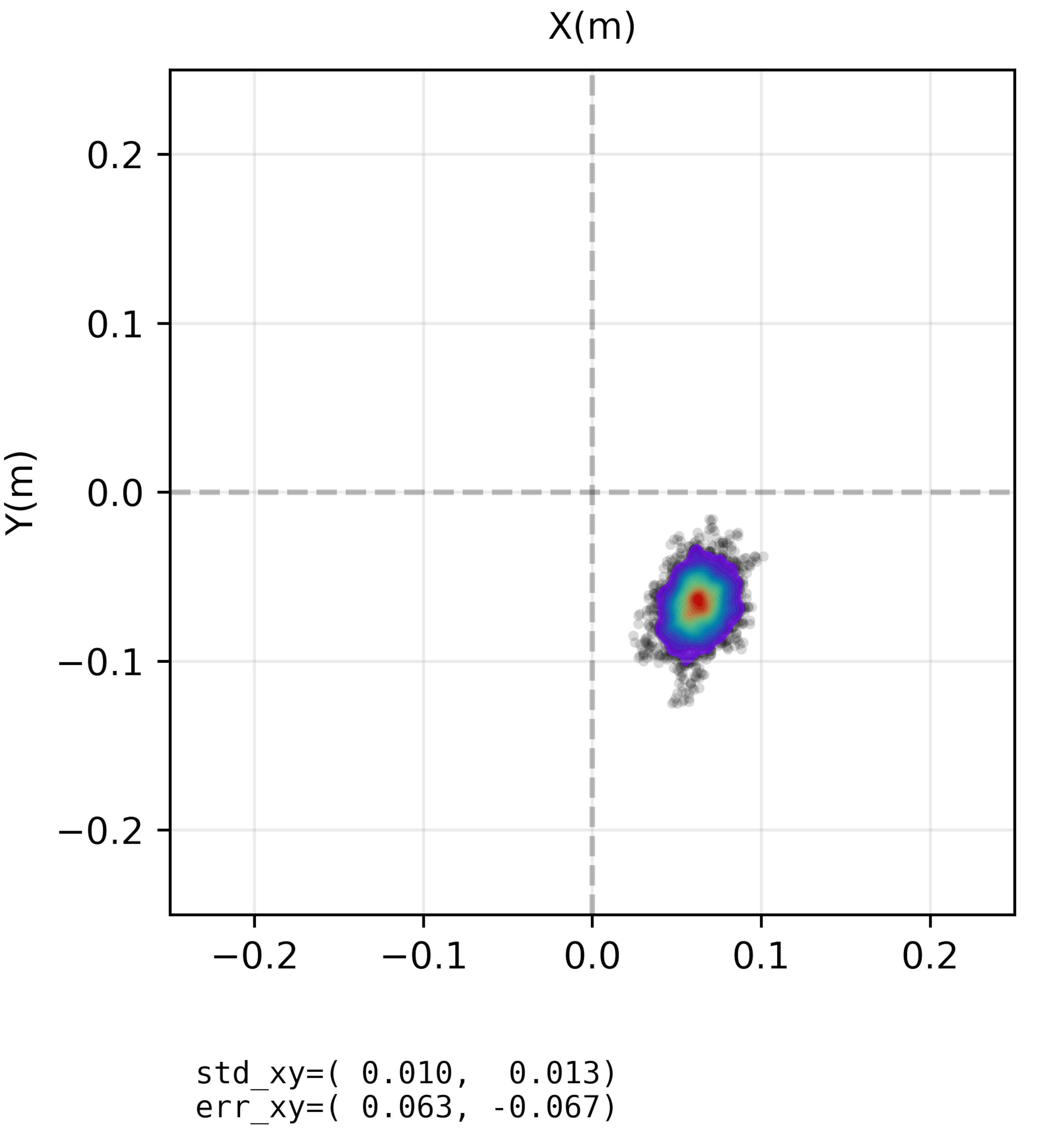
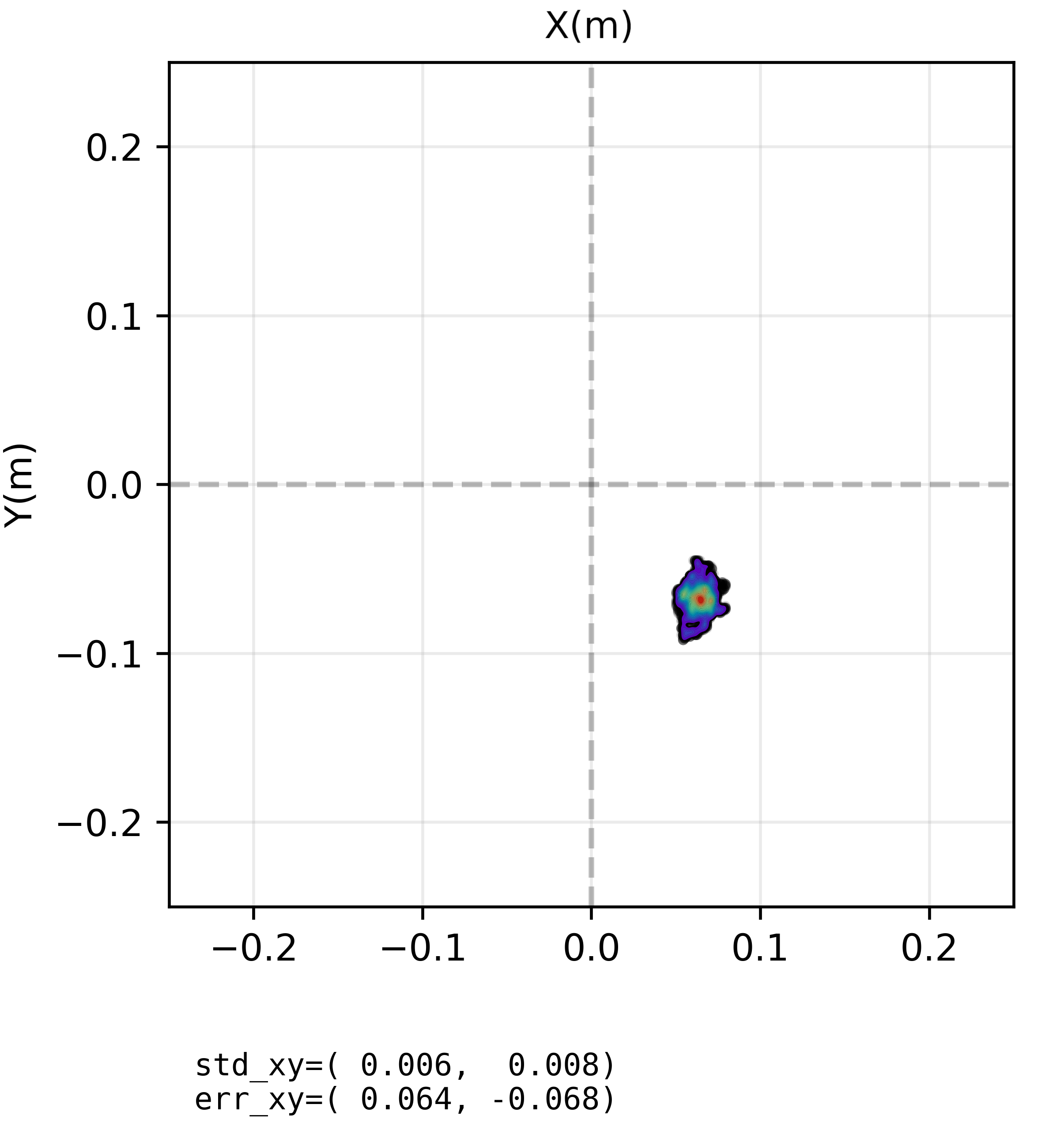
| No smoothing applied | 10 smoothing | 100 smoothing |
In the figures above, we observe a Tag with a raw precision standard deviation (σ) of approximately 2.4 cm in the X-axis and 2.3 cm in the Y-axis when tracked by six Anchors in Channel 9 Multi-Time mode at 100 Hz update rate. This standard deviation is representative of many high-performance CUWB installations. In the test setup, this Tag remains stationary for the duration of the test while varied smoothing levels are applied and the resultant standard deviation is recorded. This Tag’s physical location is (0.004 m, 0.006 m).
| Samples Smoothed | Smoothed Rate1 | Calculated Standard Deviation | Measured Standard Deviation (X-Axis) |
|---|---|---|---|
| 1 (Raw Data) | 100 Hz | - | 2.4 cm (0.024 m) |
| 10 | 10 Hz | 0.76 cm (0.0076 m) | 1.0 cm (0.010 m) |
| 100 | 1 Hz | 0.24 cm (0.0024 m) | 0.6 cm (0.006 m) |
1. When using smoothing, the CUWB System delivers output data at the nominal configured rate while smoothing the last N-samples on a sliding window. A user needing the ‘equivalent rate’ to meet latency requirements for their system can run at a higher rate, smooth N samples, and achieve better precision without sacrificing latency.
Applying N=10 smoothing reduces the real-world standard deviation to 1.0 cm. Further increasing to N=100 smoothing achieves a real-world standard deviation of 0.6 cm, demonstrating a consistent and significant reduction in standard deviation as smoothing is increased.
The CUWB Series 300 supports high Tag beacon rates. This allows deployments to apply aggressive smoothing algorithms to reduce positional jitter while maintaining the responsiveness required for high-speed tracking. See Tag Roles for instructions to set up beacon rates for Tags.
Anchor Density
Another important factor for performance is the number and placement of Anchors participating in the solution.
Anchor Utilization
A typical UWB RTLS uses triangulation or trilateration, which limits the total number of Anchors included in the output solution. When additional Anchors are available, the system must address the overdetermined solution.
The CUWB Engine consumes data from all Anchors that detect a Tag, including Quiet Anchors, and processes the data simultaneously in one pass of the algorithm. There is no practical upper limit to the number of Anchors that can contribute to the solution, allowing system precision to improve as additional Anchors are added. For more information, see APD001.
Weighting Optimization
The CUWB Engine applies advanced weighting algorithms to the underlying timing data received from each Anchor. Anchors providing high-quality measurements and favorable geometry are prioritized, while Anchors with weak or noisy data are de-weighted. This ensures the solution is always driven by the best available data. For more information, see APD001.
Resilience and Occlusion
High Anchor density also provides resilience against environmental occlusions. In a warehouse environment, a forklift may temporarily block the LoS to five Anchors. In a sparse system, this could result in a complete loss of tracking or a significant position jump. In a high-density deployment, eight to fifteen other Anchors are likely to maintain a clear view, allowing the CUWB Engine to continue tracking without interruption. See the Component Placement Guide for Anchor and Tag placement considerations.
Geometric Dilution of Precision (GDOP)
GDOP is a multiplier of error based on geometry. If Anchors are clustered together or form a straight line, the intersection of their position measurements becomes elongated and uncertain.
By increasing the number of Anchors and placing them strategically around the tracking area, GDOP improves and precision uncertainty decreases. This locks the Tag position into a tighter best-fit position, significantly reducing the geometric amplification of error.
Measured Performance - Anchor Count
To demonstrate the impact of spatial density on precision, we analyzed the same static Tag referenced earlier solved with varying numbers of participating Anchors. The data below reflects raw position measurements (no smoothing) to isolate the effect of Anchor count.
 |
|---|
| XY Position Data for 01:12:007F |
- 6 Anchors: With a minimal Anchor set, the raw position shows a standard deviation of approximately 2.4 cm in X and 2.3 cm in Y.
- 12 Anchors: Doubling the participating Anchors significantly reduces noise. Standard deviation drops to 1.5 cm in X and 1.4 cm in Y.
- 24 Anchors: Utilizing 24 Anchors refines the raw precision to sub-centimeter levels in the horizontal plane with standard deviations of 0.8 cm in both X and Y.
Increasing the number of Anchors can also improve the accuracy of the system. Our example Tag’s average position error (accuracy) improves from 6.3 cm in the X-axis and 6.8 cm in the Y-axis when tracked by six Anchors, to 3.1 cm and 1.6 cm, respectively, when tracked by 24 Anchors.
High Performance Configurations
A compromise exists between Anchor density and the degree of smoothing applied. Utilizing a higher Tag update rate that is subsequently smoothed can, to some extent, permit an installation with a reduced Anchor count.
CUWB deployments requiring extremely high precision often utilize both smoothing and high Anchor densities. For our example Tag, tracked with 24 Anchors and 100 smoothing, the standard deviation was 3 mm or less in the X and Y axes.
| Anchor Count: | Smoothing: | Measured Standard Deviation X | Measured Standard Deviation Y | Measured Error in X | Measured Error in Y |
|---|---|---|---|---|---|
| 6 | 1 (Raw Data) |
2.4 cm (0.024 m) |
2.3 cm (0.023 m) |
6.3 cm (0.063 m) |
-6.8 cm (-0.068 m) |
| 12 | 1 (Raw Data) |
1.5cm (0.015 m) |
1.4 cm (0.014 m) |
3.6 cm (0.036 m) |
-2.7 cm (-0.027 m) |
| 24 | 1 (Raw Data) |
0.8 cm (0.008 m) |
0.8 cm (0.008 m) |
3.1 cm (0.031 m) |
-1.6 cm (-0.016 m) |
| 6 | 10 | 1.0 cm (0.010 m) |
1.3 cm (0.013 m) |
6.3 cm (0.063 m) |
-6.7 cm (-0.067 m) |
| 12 | 10 | 0.6 cm (0.006 m) |
0.8 cm (0.008 m) |
3.8 cm (0.038 m) |
-2.4 cm (-0.024 m) |
| 24 | 10 | 0.4 cm (0.004 m) |
0.5 cm (0.005 m) |
3.2 cm (0.032 m) |
-1.8 cm (-0.018 m) |
| 6 | 100 | 0.6 cm (0.006 m) |
0.8 cm (0.008 m) |
6.4 cm (0.064 m) |
-6.8 cm (-0.068 m) |
| 12 | 100 | 0.4 cm (0.004 m) |
0.6 cm (0.006 m) |
3.7 cm (0.037 m) |
-2.3 cm (-0.023 m) |
| 24 | 100 | 0.2 cm (0.002 m) |
0.3 cm (0.003 m) |
3.3 cm (0.033 m) |
-1.9 cm (-0.019 m) |
System Design Trade-offs and Mitigations
While increasing beacon rates and Anchor density improves performance, these choices introduce specific trade-offs that must be accounted for during the planning phase.
Beacon Rates vs Capacity
The CUWB System has a finite capacity, measured in Locates per Second (LPS). Increasing the beacon rate of individual Tags consumes this budget, reducing the total number of Tags the system can support.
- High Capacity Scenario: A warehouse tracking 3,000 pallets may run Tags at 1 Hz to maximize the device count.
- High Precision Scenario: A robotics lab tracking 30 AGVs may run Tags at 100 Hz to maximize precision while maintaining responsiveness.
Users must balance the required precision of the tracking against the total population of Tags in the zone.
It should be noted that Tags in the CUWB System can operate at different beacon rates and can also be switched between them dynamically. Some users employ geofencing techniques to optimize this trade-off by moving Tags between Roles with different beacon rates based on their physical locations. See our American Football Deployment as an example of this use case.
Anchor Density vs Infrastructure Cost
Increasing Anchor density directly increases hardware and installation costs. More Anchors require additional cabling, switch ports, and installation labor. The CUWB System mitigates much of this trade-off with its ChainPoE(™) technology and flexible mounting options. Designers should also consider zoning their Anchor density. It is often efficient to deploy a sparse Anchor array grid for general tracking areas and increase density only in critical zones where improved precision is required.
Conclusion
The performance of a CUWB deployment is an outcome of intentional system design, implementation, and configuration rather than a static hardware specification.
By adjusting the primary design levers, users can tailor the CUWB environment to their specific application objectives:
- To Maximize Precision and Accuracy: Increase Anchor density and utilize high Tag beacon rates. This provides the CUWB Engine with more data for the location solution and enables aggressive mathematical smoothing to achieve sub-centimeter precision.
- To Maximize Capacity: Reduce Tag beacon rates to minimize airtime utilization. This allows the system to support the largest possible population of concurrent Tags within a single zone.
- To Minimize Cost: Deploy sparse Anchor arrays, particularly in non-critical zones. This is a cost-effective solution for general tracking where lower precision and reduced occlusion resilience are acceptable.
The question is not “How precise is the system?” but rather “What configuration provides the required accuracy and precision for this application?” By treating these factors as design variables, users can optimize their CUWB deployment to balance performance, capacity, and budget.
Revision
| Version | Date | Change Description |
|---|---|---|
| 5.1.0 | 2026-05-01 | Revised document sections, updated images, added empirical data examples |
| 5.0.0 | 2026-02-10 | Initial Preliminary Release |